[Tutorial] MarsGan - How to generate synthetics images of Mars' surface using StyleGAN
- 23 minsHow to generate synthetics Mars’ surface images using StyleGAN
If we are asked to draw a picture of the surface of Mars, we will probably draw a reddish surface, perhaps with a crater or some other geographical feature. Although the surface may be more complex, and have various colors and distinct shapes, minerals and characteristics, we agree that we can characterize the visual properties of the surface. If we were really good enough drawers and knew the properties of the surface of Mars well enough, we could generate fake images that would even fool a specialist, since the properties of the images would be the same as a real image and the quality of the image would be the same.
Generative Adversarial Networks (GANs) are a neural networks that are composed by two networks: a Generator network -the artist- and a Discriminator network -the specialist- which are trained in a two player game. The generator (the artist) tries to fool the discriminator by generating real looking images, and the discriminator (the specialist) tries to distinguish between real and fake making the generator to do its best to fool the discriminator. If we iterate over this game with enough fake and real examples, the generator will learn how to synthesize fake images that have the same statistics or properties as the real images and fool the discriminator.
In this tutorial we will see how to train a GAN developed by Nvidia, the StyleGAN, to exploit this idea and generate synthetic images of Mars’ surface which look like real ones. The aim of this tutorial is to show hot to train end-to-end a GAN to generate good quality synthetic images and discuss some things of the pipeline. I will assume that you know some basic concepts about machine learning and some basic python stuff.
I strongly recommend to read some theory or material about generative models and GANs because it is fascinating and revolutional, in fact Yann LeCun described GANs as the coolest idea in machine learning in the last twenty years.
Teaser
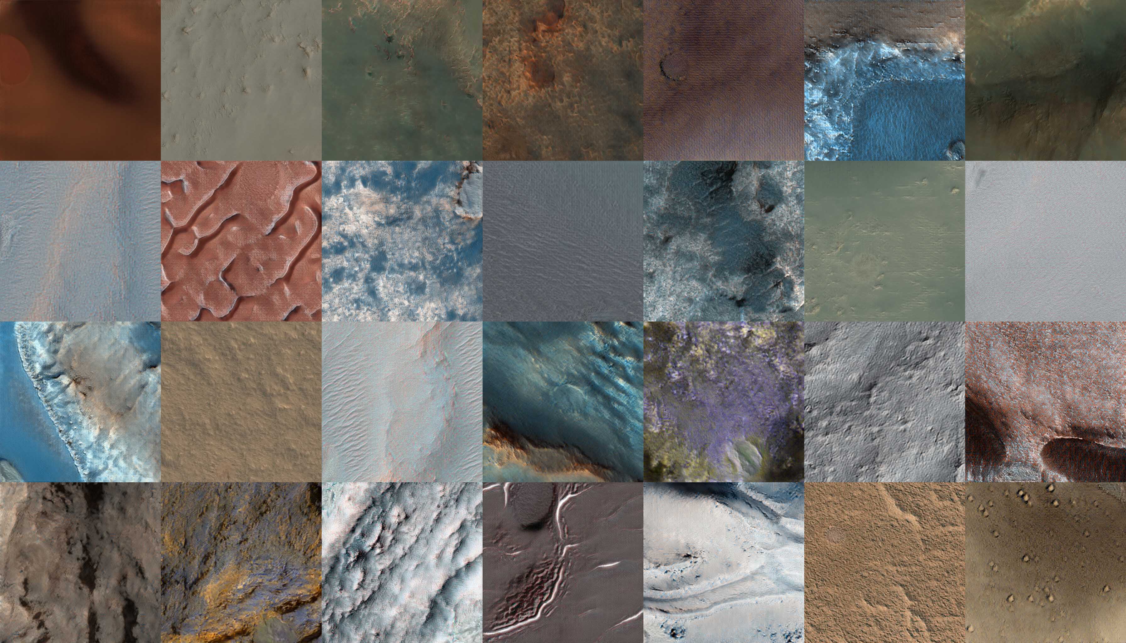
Fake or real?
Synthetic images
Real images
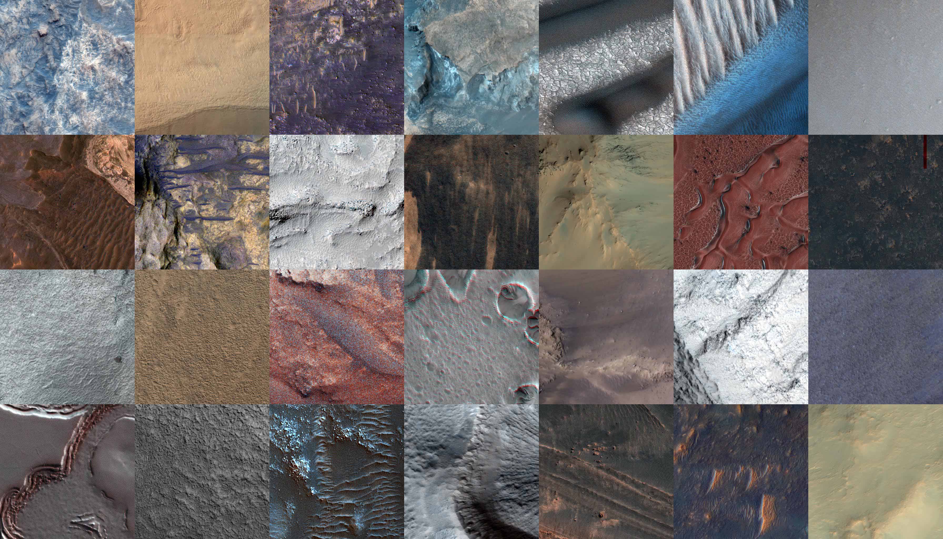
Can you tell the difference?
Training evolution (it may take a while to load ~18Mb), click to view the full video. 
Some useful theoretical resources
- A ver nice tutorial to play with and get some intuition about these concepts
- Ian’s Goodfellow -the creator of GANs- tutorial
- Stanford Lecture about generative models
Now, let’s get started!
Requirements
- Linux, MacOs or Windows are supported, but I strongly recommend to use Linux.
- One o more GPUs with that support CUDA with at least 8Gb of RAM.
- 64-bit python.
Useful resources:
- CUDA installation https://developer.nvidia.com/cuda-downloads
Generating the training set
Obtaining the raw images
As in every machine learning pipeline, we need a training dataset to train our GAN. We will use images provided by HiRISE (High Resolution Imaging Science Experiment), which is the the most powerful camera ever sent to another planet. In the catalog of HiRISE there are lots of images that look like these
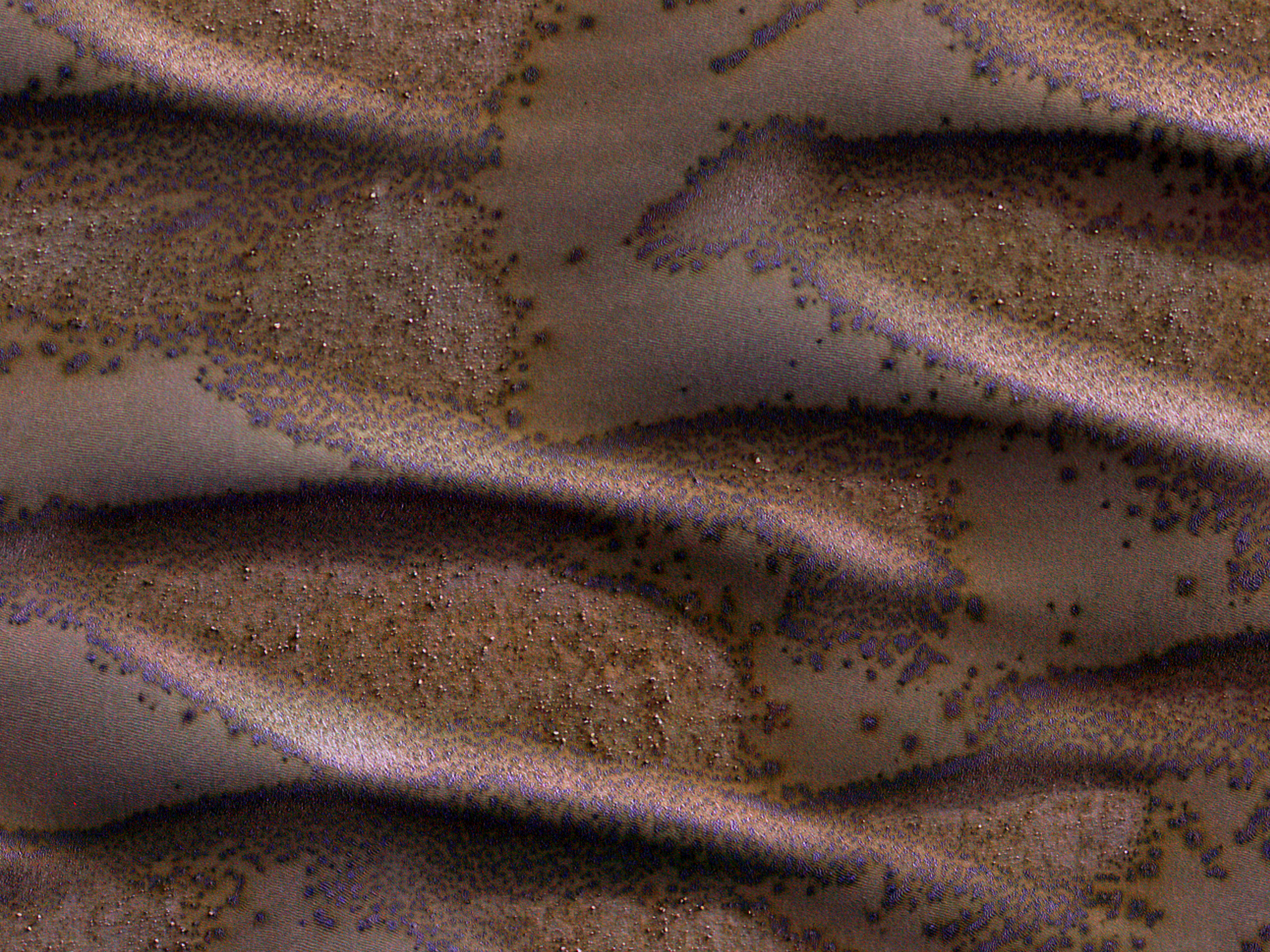
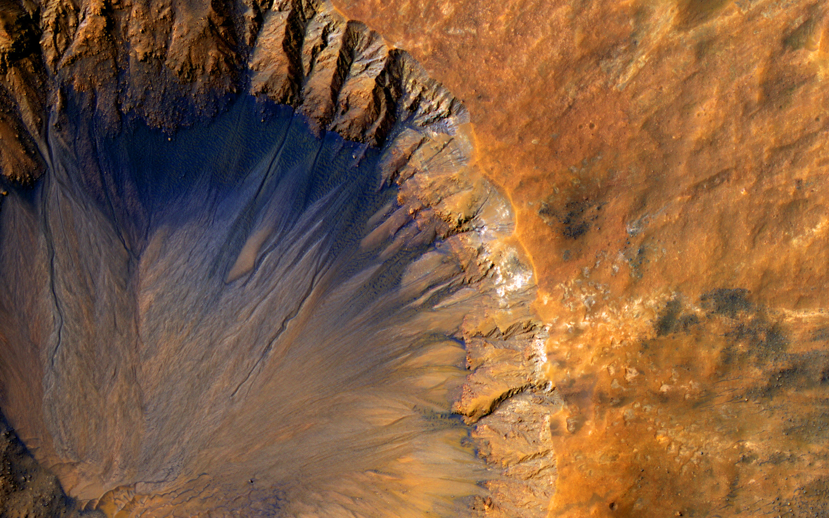
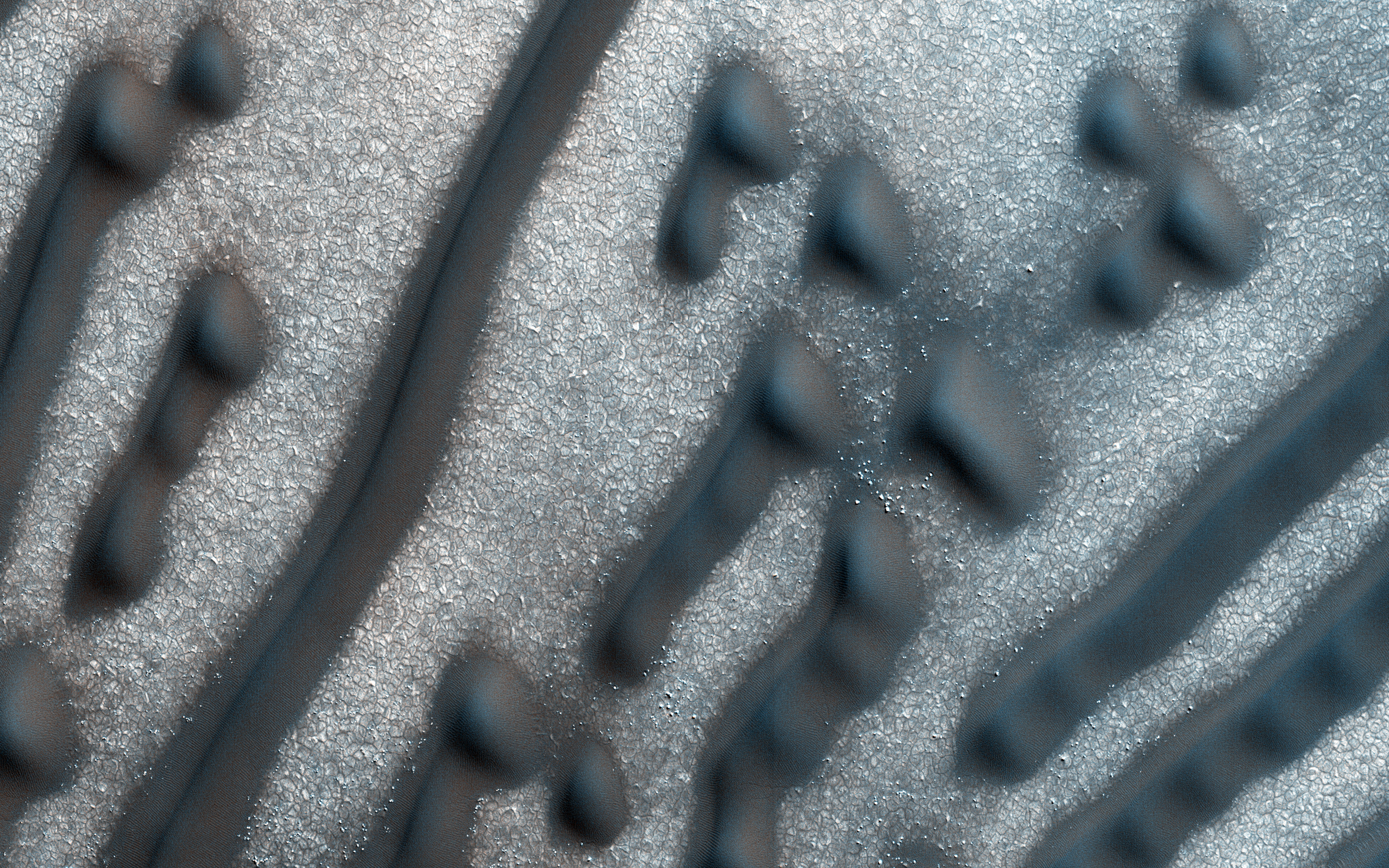
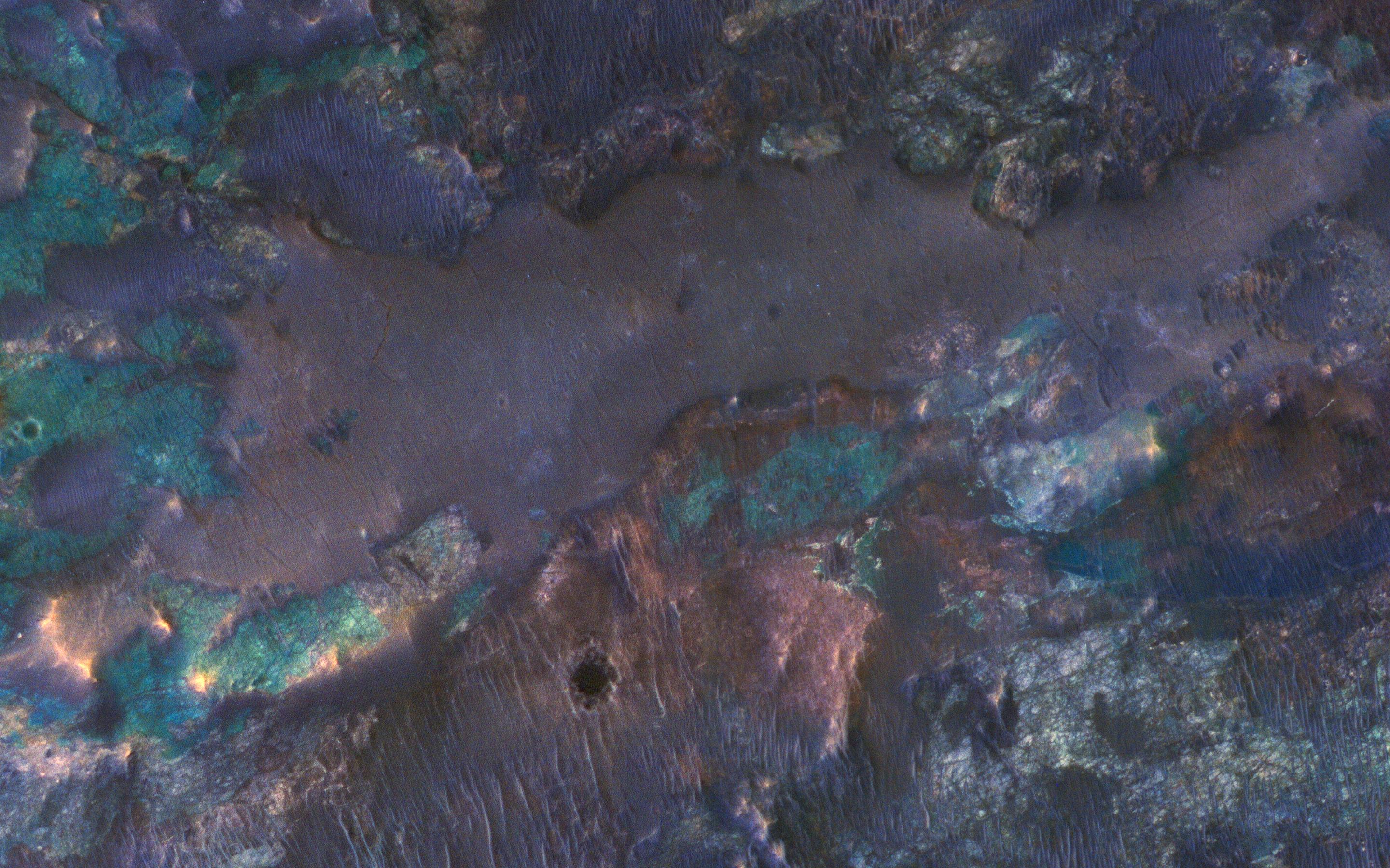
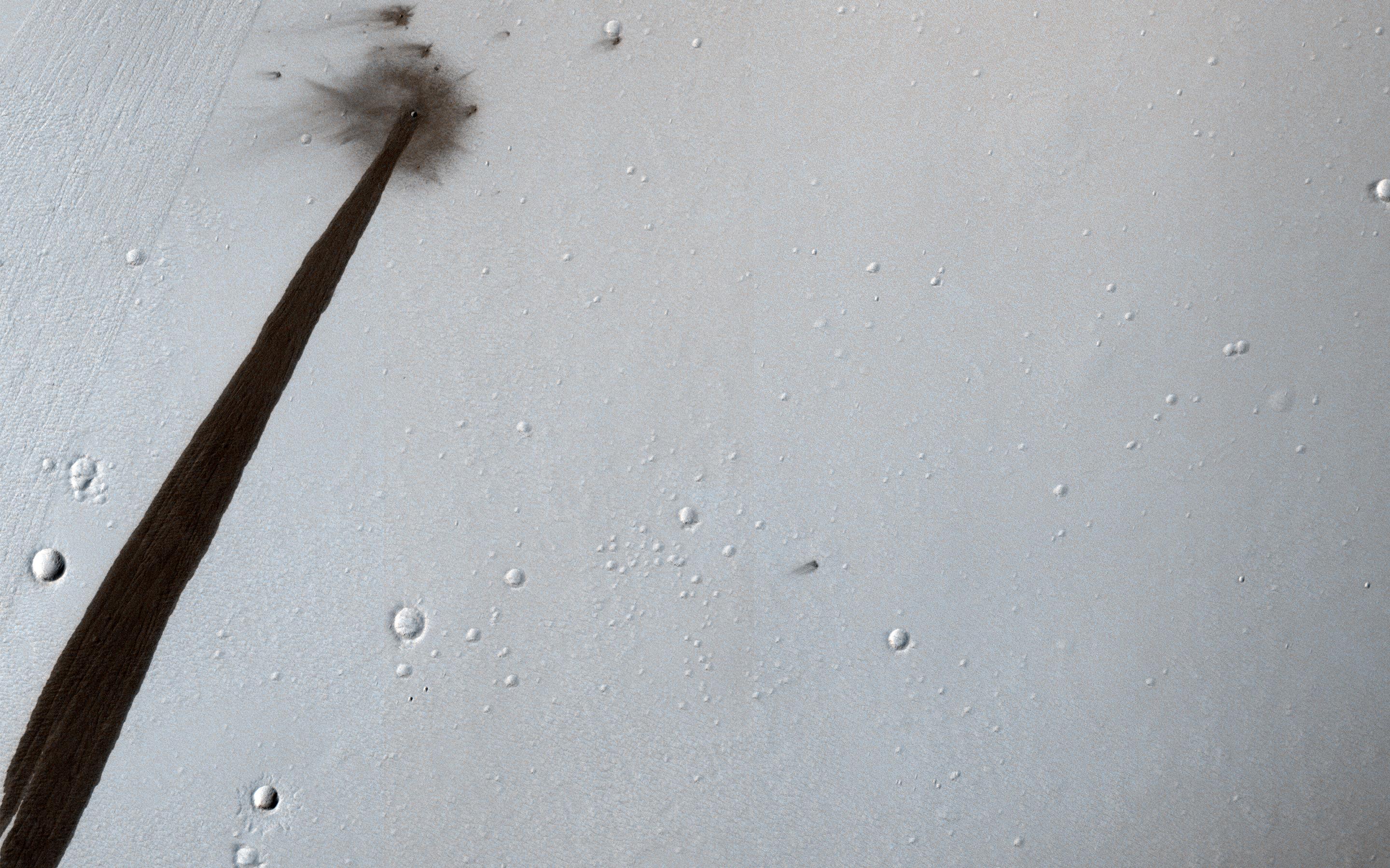
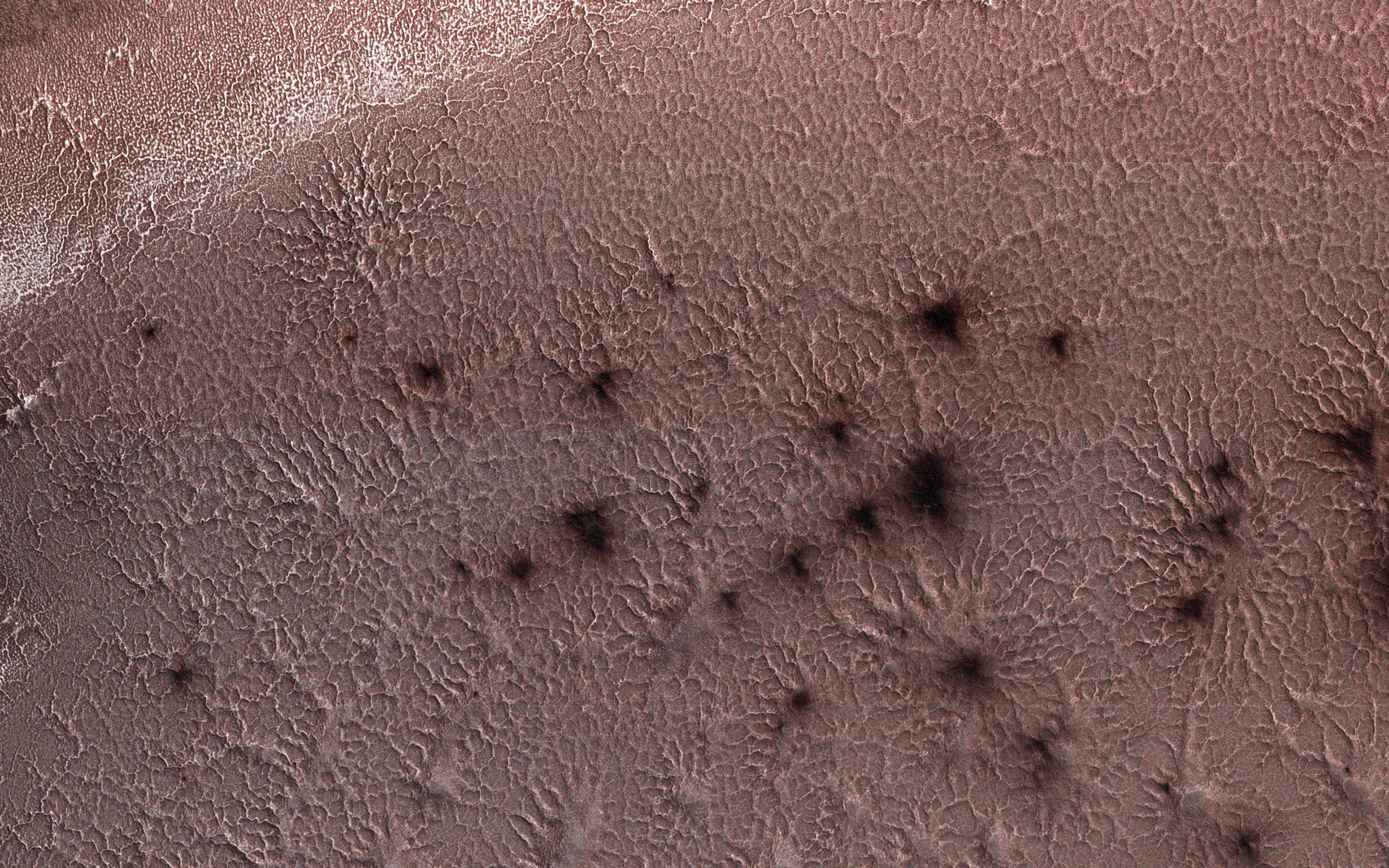
I have to say that at the beginning I was not planning to make a MarsGAN, however after seeing this images that look almost as a Sci-Fi movie, the first thing that came to my mind was in trying to train something with the images. The rest of the story is this tutorial…
To download the images go to the catalog, open an image that you like and then for example this one, and download the IRB-color non-map image, which are all jpg images.
There are different time of images, some of them are wallpapers, some others are very tall ones, and also there are different sizes. Download as many as you can and for the moment do not worry about the different shapes of the images. Then we are going to process the images so they all have the same shape. In this tutorial the images that we are going to generate are of 512x512 px size, so the only consideration that you have to take care is that the smaller dimension of the images must be at least 512px.
So, after a couple of downloads my raw dataset consists of 344 jpg images of the database and drop them all in the same folder, in my case is the /datasets/raw folder.
.
└── datasets
    └── raw
Creating a python environment (move before data creating the dataset)!
We will install several packages to be able to train the GAN and some of them need specific versions and we don’t want to interact or change the version of other packages. Thus, to keep on we need to setup the python virtual environment.
A virtual environment is a tool that helps to keep dependencies required by different projects separate by creating isolated spaces for them that contain per-project dependencies for them.
Basically by using a virtualenv we can install a lots of packages and even broke the environment without damaging other python installations or changing the versions of other packages in other environments. I strongly recommend using anaconda -aka conda-, since it is very easy to install python and setup a virtual environment with conda. In particular I suggest installing the miniconda version which has the minimal components, and is quite faster. Follow these steps to install anaconda on your OS or these steps to install miniconda. If everything worked find you will be able to use the conda command in your terminal with either of the two installations.
$ conda V
conda 4.5.11
Next we create a python environment using conda. You will be asked to accept and install some python packages.
$ conda create --prefix ./stylegan_env python=3.7
After the creation of the environment you will find a new folder.
.
└── datasets
│   └── raw
└── stylegan_env
    ├── ...
    ...
To activate the environment
~/stylegan_tutorial $ conda activate ./stylegan_env
(/home/ivan/stylegan_tutorial/stylegan_env)
~/stylegan_tutorial $
(To deactivate the environment the command is conda deactivate.)
Installing dependencies
Having the virtualenv activated, we will install the dependencies needed to train the GAN.
$ conda install six pillow requests
The implementation that we are going to use of StyleGAN was released for the version 1.10.0 or higher (still 1.x) of tensorflow. Nowadays tensorflow already has released the 2.x version that has some changes that will make the tutorial a little bit harder to follow. Thus, we are going to install the last 1.x version.
$ conda install tensorflow-gpu==1.14.0
Now that we have the environment ready we are ready to run some code. I hope that I dind’t forget any package here, but if I did, just conda-install it.
Preparing the dataset
Converting images to RGB
If by any change you download a couple of images that are in black and white or have the wrong RGB format, we are going to standardize the dimension of all the images.
Removing the borders
You might find lots of images that have a red border like this one. Although this border might represent less than the 0.1% of the image, I don’t want to include this part of the image since it may introduce noise to the dataset.  So I will move all 133 the images that contain borders to
 './raw/with_borders/'. Then I will run this simple script that you can run either on jupyter or as a python script:
After this procedure the raw images will no longer have the upper border.
Finally we can now add the images that have no border to './datasets/curated/'. My whole raw dataset consists of 343 images, and their sizes range from 512px, 10459px to 1328px, 1184px
.
└── datasets
│   ├── curated
│   └── raw
│       └── no_border
└── stylegan_env
    ├── ...
    ...
More preprocessing - data augmentation
To be able to use the images that we have, first we need to reshape the images into a square shape; in general GANs use square images. For this particular tutorial we are going to cut the raw images into images of size 512px x 512 px. This size will generate high quality images and the training process is not going to be SOOOO long. If you have lots of GPU or time, you can try generating 1024px x 1024 px, I am confident that you will have good results. The bigger the images sizes, the larger the dataset that you will need to train the GAN. As a starting point I suggest trying 128px x 128px, with this size you will train considerable faster the GAN compared to 512px x 512 px. I used a NVIDIA Titan V, and I took me 2 days of training for the 128px x 128px and around 12 days for the 512px x 512 px images. Yes, I know, this sounds like a lot of time, but training GANs takes a lot of time. It is important to note that whichever size you choose it must be a multiple of 2. Additionally we are also to make some data augmentation.
So, now we are going to cut into 512px x 512 px pieces all the raw images. And we define some functions that we are going to use also for the data augmentation.
Data augmentation is a strategy that enables practitioners to significantly increase the diversity of data available for training models, without actually collecting new data.
Training deep learning neural network models on more data can result in more skillful models, and the augmentation techniques can create variations of the images that can improve the ability of the fit models to generalize what they have learned to new images.
In this particular case we are going to rotate and flip the images in different directions. For satellite images this procedure will work well because we expect that the properties of the images that we want the GAN to learn, do not change when the image is rotated. For example, a crater will still be a crater even though we rotate or flip the images. In other cases, for example faces or landscapes, we have to be more careful because we don’t want to generate upside down faces or portraits. Data augmentation, or image augmentation, has to keep the properties of the images unchanged under the transformations that we make to the images.
So first if we only cut the images into (512, 512) images we obtain 4120 images. After the augmentation we in which we keep the original + 4 transformations we have 5 * 4120 = 20600 images. For this dataset this number is enough.
.
└── datasets
│   ├── curated
│   ├── cropped_files_aug
│   ├── cropped_files_no_aug
│   └── raw
│       └── no_border
└── stylegan_env
    ├── ...
    ...
I wrote my own augmentation scripts because I don’t need a huge increase in the data set, and just some simple transformations are enough. But if you want to see which kind of techniques are use for image augmentation you can checkout this links.
Some more data augmentation resources:
- https://towardsdatascience.com/data-augmentation-for-deep-learning-4fe21d1a4eb9
- https://keras.io/preprocessing/image/
- https://machinelearningmastery.com/how-to-configure-image-data-augmentation-when-training-deep-learning-neural-networks/
–>
So for the moment we have around 20k 512, 512 pxs images ready to be used to train the GAN.
In the next steps we are going to implement the StyleGAN, so before we move on I strongly recommend reading the StyleGAN README. You don’t need to understand everything but you will gain some intuition at least.
Clone the StyleGAN repository
So, now we need to clone the StyleGAN repository where you will find the tensorflow implementation of the StyleGAN. One option is to download directly the repo from github, the other one is to clone it using git
Using git:
git clone https://github.com/NVlabs/stylegan.git
.
└── datasets
│   ├── curated
│   ├── cropped_files_aug
│   ├── cropped_files_no_aug
│   └── raw
│       └── no_border
├── stylegan
└── stylegan_env
    ├── ...
    ...
Create tensorflow records
Next we need to create tfrecords from our data set. From the StyleGAN github:
The training and evaluation scripts operate on datasets stored as multi-resolution TFRecords. Each dataset is represented by a directory containing the same image data in several resolutions to enable efficient streaming. There is a separate *.tfrecords file for each resolution, and if the dataset contains labels, they are stored in a separate file as well.
$ cd stylegan
$ python dataset_tool.py create_from_images datasets/mars ../datasets/cropped_files_aug
At the path datasets/mars there are going to be several files, each corresponds to a different resolution. The training is progressive, first it starts with low resolution images and then it increases till the final size.
Train
Setup train.py
Now we are very close to start our training. To setup the configuration of the training we need to modify the file stylegan/train.py.
- We have the tfrecords as our dataset. We do this by removing this ine
desc += '-ffhq'; dataset = EasyDict(tfrecord_dir='ffhq'); train.mirror_augment = Trueand replacing it with this one
desc += '-mars'; dataset = EasyDict(tfrecord_dir='mars'); train.mirror_augment = False - We need to specify the number of GPUs that we are going to use. In my particular case I only have one GPU. I commented this line
desc += '-8gpu'; submit_config.num_gpus = 8; sched.minibatch_base = 32; sched.minibatch_dict = {4: 512, 8: 256, 16: 128, 32: 64, 64: 32}and uncommented this one
desc += '-1gpu'; submit_config.num_gpus = 1; sched.minibatch_base = 4; sched.minibatch_dict = {4: 128, 8: 128, 16: 128, 32: 64, 64: 32, 128: 16, 256: 8, 512: 4} - Finally I changed the number of images that I used in the training set. In my particular case they are 20600 images. So I changed the number 25000 to 20600 in this line.
train.total_kimg = 25000train.total_kimg = 20600
The other default parameters worked fine for me. So now we are ready to go!
Train the GAN
The training is progressive. This means that it will start with low size images and it will progressively start to increase the size of the images till it reaches the final size. The first epochs with small probably will finish quickly, but don’t get excited to fast, because as soon as the images increase their size you will notice the difference. I remind that for 20600 images of 512px it took more than ten days of training. So, be patient…
To start the training be sure to have active the virtual env that you created for this project and just run
python train.py
and voilà! The train will start.
You will see some prints with the summary of the architecture of the network, and finally a message saying Training.... Now we are done.
Every time an epoch has finised you will see a message like this one:
tick 1 kimg 140.3 lod 6.00 minibatch 128 time 3m 36s sec/tick 163.2 sec/kimg 1.16 maintenance 52.8 gpumem 3.8
If you think that the training is not running and you have an NVIDIA GPU you can run the command nvidia-smi to monitor the state of the GPU.
Checkout the training progress.
The train script save some snapshots during the training to show you the progress of the training. You can check them out in stylegan/results/00001-sgan-mars-1gpu/. You will find network snapshots network-snapshot-****.pkl from which you can resume the training, and also synthetic samples fakes****.png.
Visualize the results and generate synthetic samples
Now that we have a trained GAN, we want to generate synthetic samples and play with the latent space.
Interpolate the latent space
Here you can find a notebook to interpolate the latent space and play with
Generate a gif of the Training
In this notebook you will find how to generate a gif from the synthetic images produced in the different stages of the training.
Outro
So that’s all folks. I will try to keep this tutorial updated for new ideas and new code. Also Nowadays NVIDIA has released the StyleGAN2, when I have some time I will add the implementation of this new GAN.
Some links, references and resources
GANs
- https://towardsdatascience.com/data-augmentation-for-deep-learning-4fe21d1a4eb9
- https://keras.io/preprocessing/image/
- https://machinelearningmastery.com/how-to-configure-image-data-augmentation-when-training-deep-learning-neural-networks/
- StyleGAN implementation
Technical stuff
- CUDA installation https://developer.nvidia.com/cuda-downloads
- Anaconda installation and miniconda installation steps.
Augmentation resources
- https://towardsdatascience.com/data-augmentation-for-deep-learning-4fe21d1a4eb9
- https://keras.io/preprocessing/image/
- https://machinelearningmastery.com/how-to-configure-image-data-augmentation-when-training-deep-learning-neural-networks/
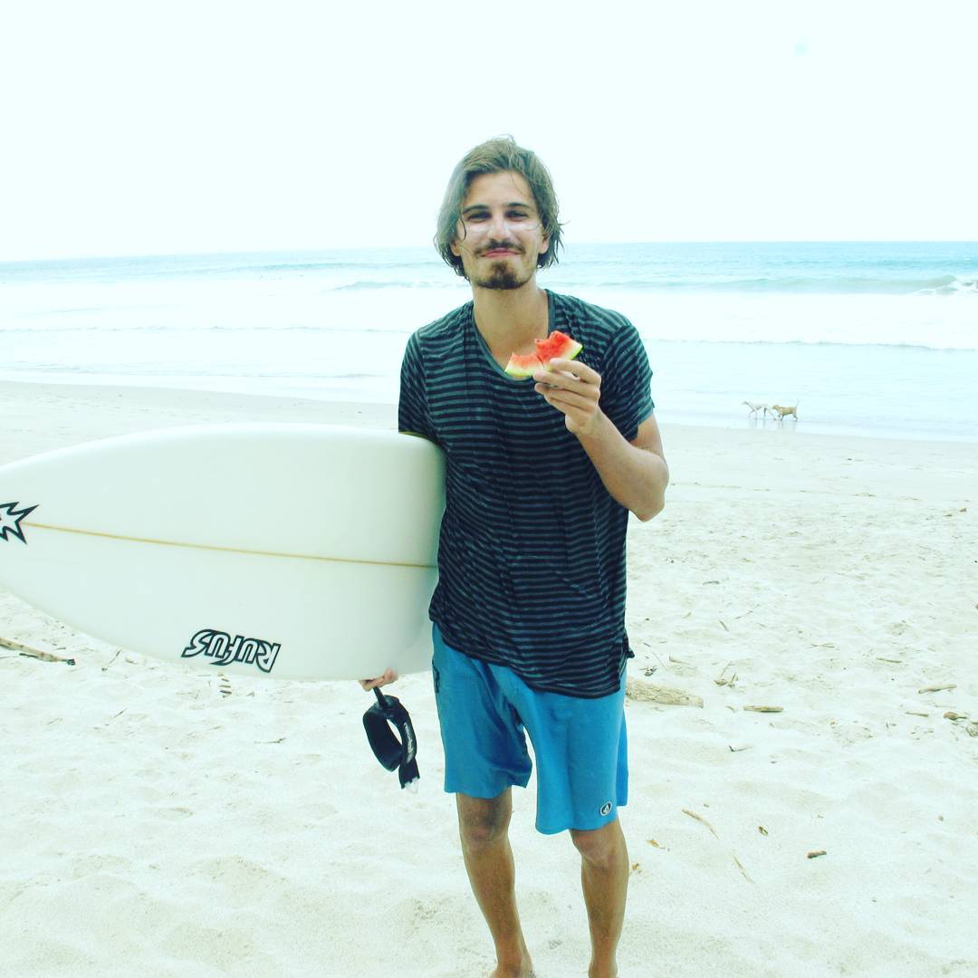
Ivan Lengyel
I wanted to be a surfer and I ended up being a nerd.